Part 4: Graphical Transformations | Beginner’s Guide Year 11 Ext 1 Maths

Do you barely function trying to figure out Graphical Transformations? In this article, we’ll walk you through Graphical Transformations so you can plot your own HSC success!

In this article, we’ll discuss:

• NESA Syllabus Outcomes
• Assumed Knowledge
• Basic Transformations
  • Shifting & Scaling
  • Reflections
  • Absolute Values
• Harder Transformations
  • Square Root and Square Transformations
  • Reciprocal Graphs
  • Addition and Subtraction Graphs
  • Multiplication Graphs
• Concept Check Questions

Year 11 Extension 1 Mathematics: Graphical Transformations

Graphical Transformations in Year 11 Maths Extension 1 builds on both prior basic polynomial sketching and sketching basic graphs in junior years.

In senior courses, being able to confidently sketch and transform a graph(s) is a key skill. These include shifting the graph, reflecting the graph, graphs involving squares and square roots and also addition, subtraction and multiplication of two functions. These will be essential skills that are necessary for applications later in Year 11 and 12, where sketching a curve enables for a visual representation of complex function problems.

Free Year 11 Maths Ext 1 Graphical Transformation

A worksheet to test your knowledge.

Download now

Free Year 11 Maths Ext 1 Graphical Transformation

Fill out your details below to get this resource emailed to you.

"*" indicates required fields

First Name*

Last Name*

Email*

Postcode*

Grade in 2025*

Grade in 2025123456789101112

Hidden

Resource (DO NOT DELETE OR CHANGE)

By submitting this form, you agree to receive promotional messages from Matrix about its products and services. You can unsubscribe at any time by clicking on the link at the bottom of our emails.

NESA Syllabus Outcomes

NESA requires students to be proficient in the following outcomes:

F1.1: Graphical relationships

• Examine the relationship between the graph of \(y=f(x)\) and the graph of \(? = \frac{1}{f(x)}\) and hence sketch the graphs (ACMSM099)
• Examine the relationship between the graph of \(y=f(x)\) and the graphs of \(y^2=f(x)\) and \(y=\sqrt{f(x)}\) and hence sketch the graphs
• Examine the relationship between the graph of \(y=f(x)\) and the graphs of \(y=|f(x)|\) and \(y=f|x| \) and hence sketch the graphs (ACMSM099)
• Examine the relationship between the graphs of \(y=f(x)\) and \(y=g(x)\) and the graphs of \(y=f(x)+g(x)\) and \(y=f(x)g(x)\) and hence sketch the graphs
• Apply knowledge of graphical relationships to solve problems in practical and abstract contexts AAM

Assumed Knowledge:

Students should have a basic understanding of curve sketching and functions. This includes having a solid grasp on the concepts of \(x\)-intercepts and \(y\)-intercepts as well as vague knowledge on the various transformations which can be applied to graphs.

This content can be found in our Year 11 Advanced Guides should students want to solidify their understanding:

• Functional Mapping

Basic Transformations

In this topic, we aim to obtain rough sketches of graphs with minimal use of calculus. In many curve sketching questions, we will not be provided with an equation. Instead we would be provided with a diagram and a generic transformation to apply. Below are the different types of basic transformations that could be asked:

• Vertical Transformations
• Horizontal Transformations
• Vertical Scaling
• Horizontal Scaling
• Reflections about the Axes
• Absolute Value Transformations

For questions which involve a mix of these transformations, always decompose the question into the basic transformations and apply in the order: horizontal changes (transformation then scaling), reflections, absolute value transformations and lastly vertical changes (transformation then scaling).

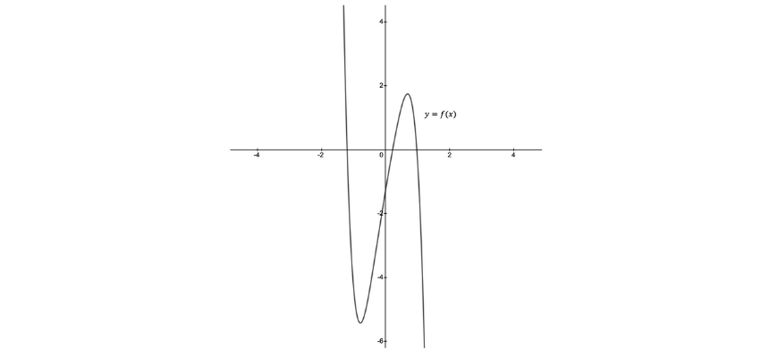
For all of our examples, we will be referencing this graph:

Vertical Transformations

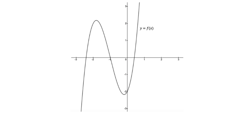
The curve given by the equation \(y = f(x)+c\), is just the curve \(y=f(x)\) shifted vertically by \(c\) units.

• If \(c>0\), the curve is shifted up by \(c\) units
• If \(c<0\), the curve is shifted down by \(c\) units

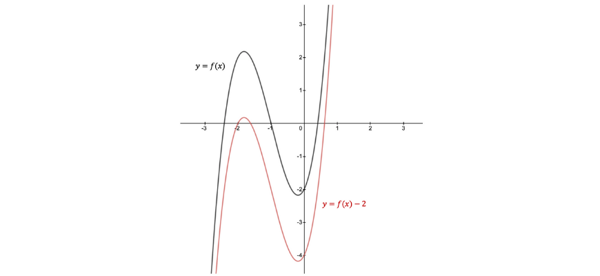
Example 1

On the axis below, draw the graph of \(y=f(x)-2\)

Solution 1

For this transformation, as \(c<0\), we shift the curve down \(2\) units:

Horizontal Transformations

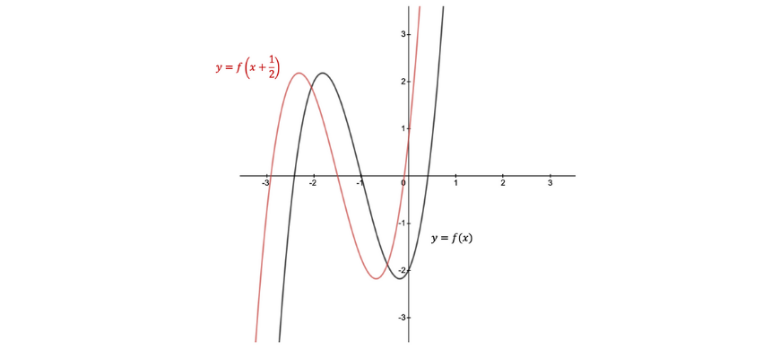
The curve given by the equation \(y = f(x-c)\), is just the curve \(y=f(x)\) shifted horizontally by \(c\) units.

• If \(c>0\), the curve is shifted right by \(c\) units
• If \(c<0\), the curve is shifted left by \(c\) units

Example 2

On the axis below, draw the graph of \(y=f(x+\frac{1}{2}\)

Solution 2

For this transformation, as \(c<0\), we shift the curve right \(c\) units:

Shifting and scaling

Vertical Scaling

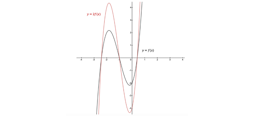
The curve given by the equation \(y = cf(x)\), is just the curve \(y=f(x)\) scaled vertically by \(c\) units.

• If \(c>1\), the curve is stretched vertically by a factor of \(c\)
• If \(c<1\), the curve is squashed vertically by a factor of \(c\)

Importantly, if the question only involves vertical scaling, only the y-intercepts are scaled, not the \(x\)-intercepts.

Example 3

On the axis below, draw the graph of \(y=2f(x)\)

Solution 3 

For this transformation, as \(c>1\), we stretch vertically by a factor of \(2\):

Horizontal Scaling

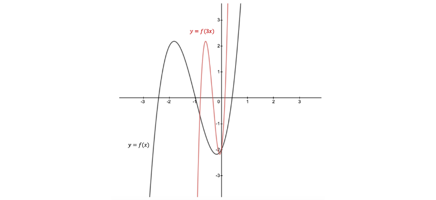
The curve given by the equation \(y = f(cx)\), is just the curve \(y=f(x)\) scaled horizontally by \(c\) units.

• If \(c>1\), the curve is squashed horizontally by a factor of \(c\)
• If \(c<1\), the curve is stretched horizontally by a factor of \(c\)

With horizontal scaling, it is a little bit more difficult as we are often going against our intuition. Importantly, if the question only involves horizontal scaling, only the \(x\)-intercepts are scaled, not the \(y\)-intercepts.

Example 4

On the axis below, draw the graph of \(y=f(3x)\)

Solution 4

For this transformation, as \(c>1\), we squash horizontally by a factor of \(3\):

Reflections

Reflections about the Axes

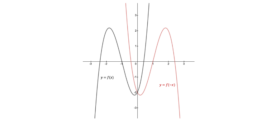
Questions which require a reflection about the axes are easily denoted by the inclusion of a negative sign:

• The curve given by the equation \(y = f(-x)\), is just the curve \(y=f(x)\) reflected about the \(y\)-axis
• The curve given by the equation \(y = -f(x)\), is just the curve \(y=f(x)\) reflected about the \(x\)-axis

Example 5

On the axis below, draw the graph of \(y=f(-x)\).

Solution 5

As we have the negative sign right next to the \(x\), this is a reflection about the \(y\)-axis:

Absolute Values

Absolute Value Transformations

There are only 2 types of absolute value transformations which can be asked in Year 11 Extension 1 Mathematics:

• \(y=|f(x)|\)
  • For this transformation, we any part of the graph which is below the \(x\)-axis is reflected about the \(x\)-axis.
• \(y=f(|x|)\)
  • For this transformation, we remove any part of the graph which is to the left of the \(y\)-axis. Then we reflect the part of the graph which is to the right of the \(y\)-axis about the \(y\)-axis.

If there is a question which requires both absolute value transformations, we always apply them in the order listed above.

Example 6

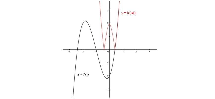
On the axis below, draw the graph of \(y=|f(|x|)|\).

Solution 6

First, we apply the \(y=|f(x)|\) transformation. Therefore, we must reflect any part of the graph which is below the \(x\)-axis:

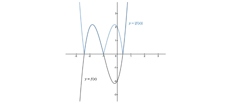
Then, we apply the \(y=f(|x|)\). Therefore, we remove any part of the graph which is left of the \(y\)-axis and reflect the part which is to right of the \(y\)-axis. This leaves us with the complete \(y=|f(|x|)|\) transformation:

Harder Transformations

Harder transformations of graphs involve graphing square roots and the addition, subtraction and multiplication of two functions. Graphing such functions can be approached by splitting the graph into segments containing key features, then combining to form the transformed graph.

Graphs of Square Roots: \(y=\sqrt{f(x)}\)

When sketching the square root of a given function, we should consider key features within the original function and how they would appear once we square root the function. Here is a reference table of the transformations to a square root function.

By splitting the graph into the ranges, we are able to sketch each segment with reference to how the features are transformed. By splitting the graph into the ranges, we are able to sketch each segment with reference to how the features are transformed.

Example 1

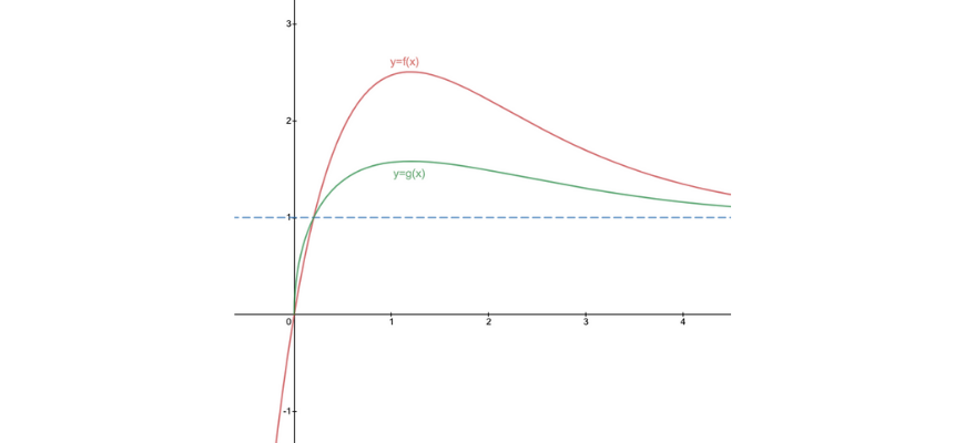
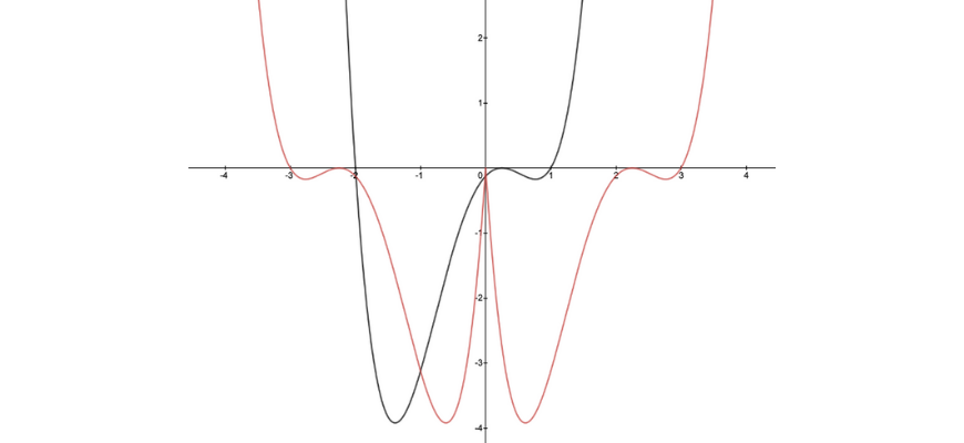
In this example, we are given \(y=f(x)\) where \(g(x)=\sqrt{f(x)}\). To approach any graph, we can split the range into 4 segments.

1. Values that have a range of less than \(0\) would not appear on our \(\sqrt{f(x)}\) graph. This is shown as the \(y=g(x)\) graph does not extend to the left of the \(y\)-axis.
2. Values between \(0\) and \(1\) would have values that are bigger than that of the original graph. This is shown by the \(g(x)\) graph being above the \(f(x)\) graph between this range.
3. Values at \(0\) and \(1\) remain the same and this is shown as an intersection between the curves at these respective points.
4. Values above \(1\) would transform into smaller values. This is shown to the right of intersection where the \(g(x)\) graph is below the \(f(x)\) graph when the range is above \(1\).

We then have to consider some key features of the graph. All increasing, decreasing portions as well as stationary points above the \(x\)-axis are retained. Asymptotes also have to be considered. From the reference table, horizontal asymptotes are square rooted. However, as the value of the asymptote is \(y=1\), this would not change.

Graphs of Squares: \(y^2=f(x)\)

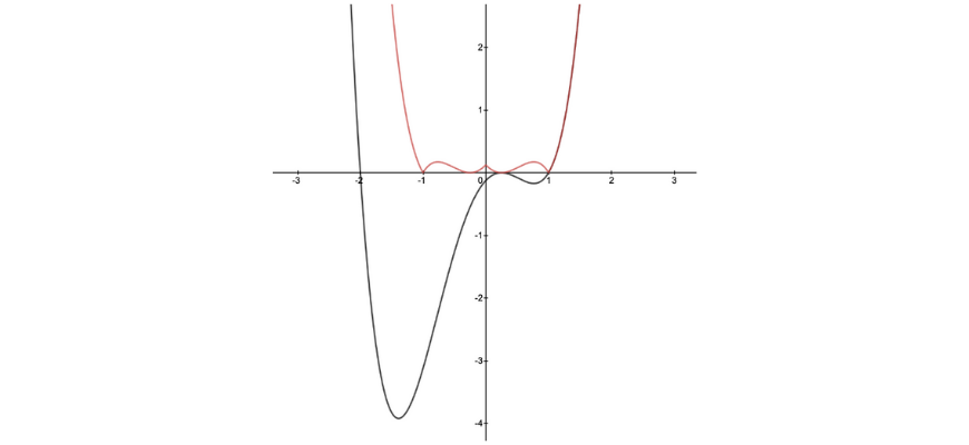
Graphing \(y^2=f(x)\) is very similar to graphing the square root graph. We can square root both sides of the equation to yield the following same result:

• \(y^2=f(x)\)
• \(y=±\sqrt{(f(x)}\)

From the previous section on reflections, we have learnt that \(y=-f(x)\) would reflect the graph along the \(x\)-axis. As the equation has both the positive and negative function, we would have the graph both.

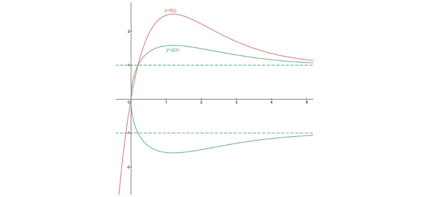
Example 2

From the example in Graphs of \(y=\sqrt{f(x)}\) to graph \(y^2=f(x)\) we would just simply add the reflection of the square root graph across the \(x\)-axis.

Note: Remember that asymptotes are also reflected and need to be shown in the graph.

Reciprocal Graphs: \(y=\frac{1}{f(x)}\)

To graph reciprocal graphs, we must first consider the key features and how these are transformed.

Example 3

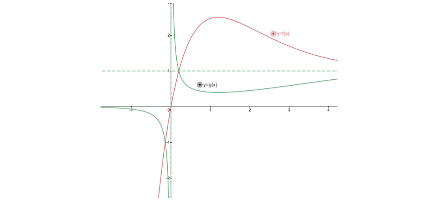
To transform the graph to its reciprocal graph, we can determine the key features and transform them before beginning to sketch.

Solution 3

\(y=f(x)\) has an \(x\)-intercept at \(x=0\). As the reciprocal produces an undefined value, this becomes an asymptote on our reciprocal graph. This has the equation \(x=0\). The horizontal asymptote should be transformed such that it is the reciprocal value. Since the equation is \(x=1\), it remains the same.

We then need to consider the limits as \(x\) approaches \(±∞\) and to the left and right of vertical asymptotes.

• As limits approach infinity, these would transform into limits approaching \(0\)
• As limits approach \(0\), these would transform into limits approaching infinity
• As limits approach a horizontal asymptotes, they would transform to limits approaching the transformed horizontal asymptote.

Taking into account that increasing values of \(f(x)\) become decreasing values of \(f(x)\) and vice versa, combined with the key features we have drawn before, we are able to construct the reciprocal graph.

Addition and Subtraction of Graphs: \(y=f(x)±g(x)\)

To graph the addition or subtraction of two functions, we firstly have to graph \(y=f(x)\) and\( y=g(x)\) separately on the same set of axes, adding coordinates. Key features that will aid us include:

Example 4

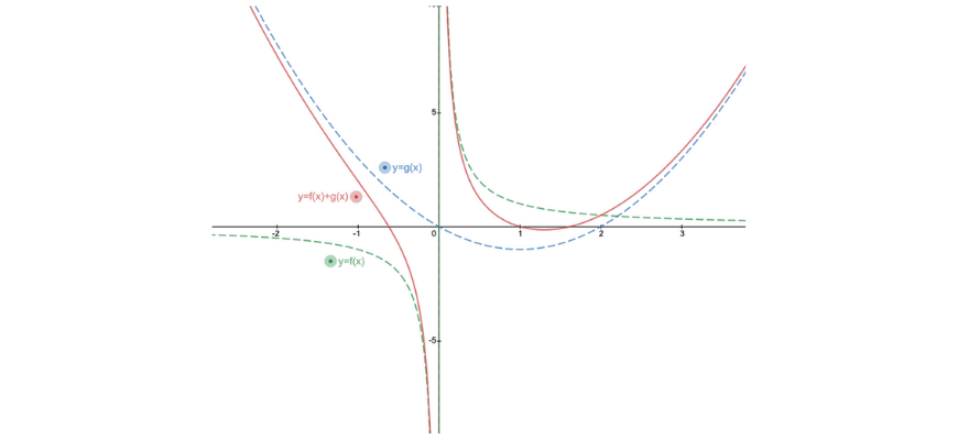
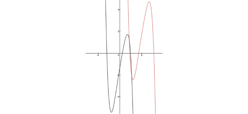
If we want to graph \(y=f(x)+g(x)\), where \(f(x)=x(x-2)\) and \(g(x)=\frac{1}{x}\), we first have to consider the key features.

Solution 4

\(g(x)\) has a vertical asymptote at \(x=0\). Therefore, we know in our addition of functions, this vertical asymptote would be translated across.

From here, we consider the \(x\)-intercepts of both graphs. On \(f(x)\), there is \(x\)-intercepts at both \(x=0\) and \(x=2\). From the reference table, if \(f(2)=0\), then \(y=g(2)\) as shown by the overlap of the green dotted line (\(y=g(x)\))and red line (\(y=f(x)+g(x)\)) in the diagram below.

We then need to consider the limits as \(x\) approaches \(±∞\) and to the left and right of vertical asymptotes.

• As limits approach infinity, if at least one function approaches infinity, then the addition of functions would be infinity. However, if one function approaches infinity whilst the other function approaches negative infinity, we have to determine which is the dominating function.
• From the graph, the following limits can be found as either function would approach a \(0\). Therefore, they would follow the limits of the function that does not appraoch \(0\).

If extra points are necessary, simply choose an \(x\) value and add the \(y\) values to achieve the addition graph.

Graphing \(y=f(x)-g(x)\) can be done in two ways.

1. Graph \(y=f(x)\) and \(y=-g(x)\) separately on the graph. Use the above rules to graph the addition of these graph.
2. Alternatively, the functions \(y=f(x)\) and \(y=g(x)\) can be graphed separately and then subtract the \(y\) values.

Multiplication of Graphs: \(y=f(x)×g(x)\)

The key features in a \(y=f(x)g(x)\) graph are outlined below

When graphing, it is important to consider the sign of the \(y\) values. For example.

\begin{align*}
&\text{Positive} \ × \text{Positive} = \ \text{Positive} \\
&\text{Positive} \ × \text{Negative} = \ \text{Negative} \\
&\text{Negative} \ × \text{Negative} = \ \text{Negative} \\
\end{align*}

Example 5

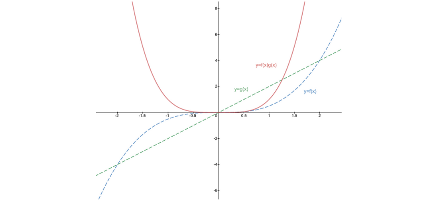
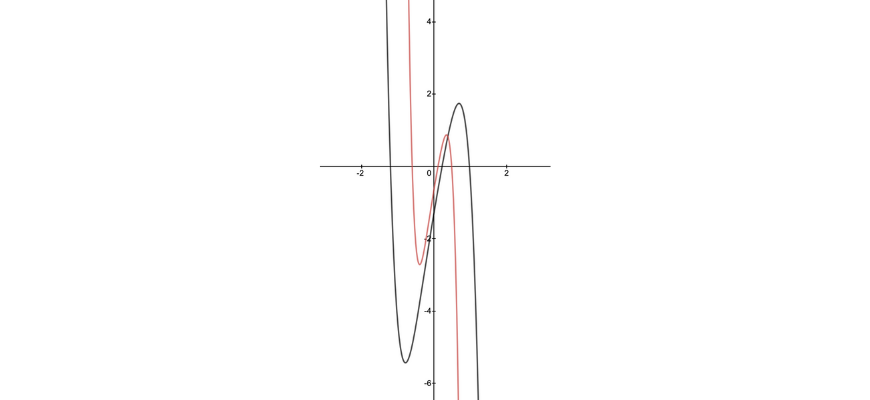
Graph \(y=f(x)g(x)\) where \(f(x)=\frac{1}{2} x^3\) and \(g(x)=2x\).

Solution 5

Similar to all harder transformation questions, we first have to graph each function individually to identify the key features. Firstly, we can identify the \(x\) intercepts of each function, as this would appear as an \(x\)-intercept on our transformed graph.

Then, we have to consider the limits as \(x\) approaches \(±∞\). From the separate graphs:

\(x→∞\),\(y→∞\)
\(x→-∞\),\(y→-∞\)

By considering the sign of each \(y\) limit, we are able to find the limit of our multiplication graph. As \(x\) approaches positive infinity, both functions approach a positive value of infinity. Therefore, this results in an infinity limit on our multiplication graph. However, as \(x\) approaches negative infinity, both functions approach negative value of infinity.

Multiplication between two negative limits would result in a positive limit as seen on the graph below.

Concept Check Questions

1. For the curve \(y=f(x)\) below, apply the following transformations:

1. \(y=f(x-2)+3\)
2. \(y=\frac{1}{2} f(2x)\)

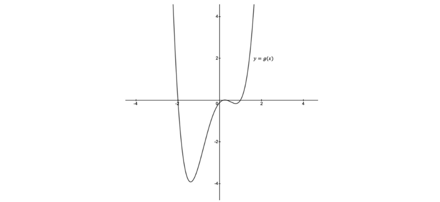
2. For the curve \(y=g(x)\) below, apply the following transformations:

1. \(y=g(|x|-4)\)
2. \(y=3|g(|x|)|\)

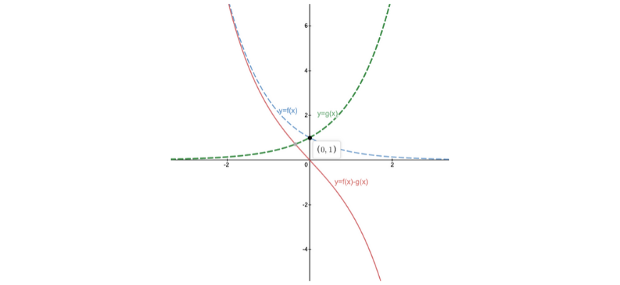
3. Graph \(y=f(x)-g(x)\), where \(f(x)=e^(-x)\) and \(g(x)=e^x\)

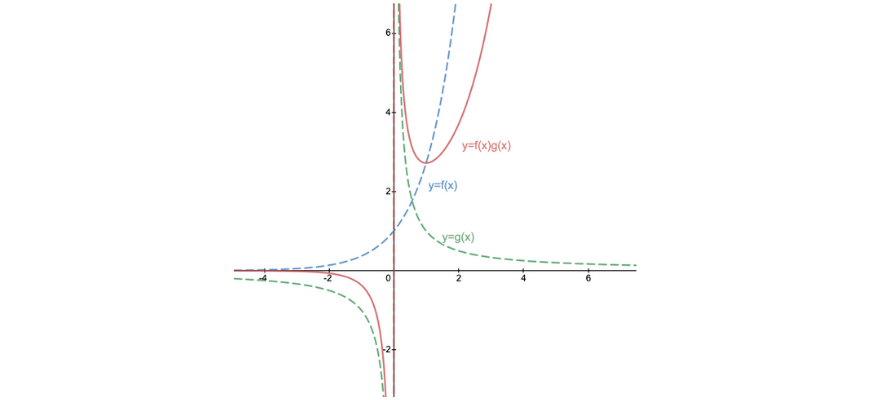
4. Graph \(y=f(x)g(x)\), where \(f(x)=e^x\) and \(g(x)=\frac{1}{x}\)

Concept Check Solutions

1.
(1)

(2)

2
(1)

(2)

3.

4.

Plot your route to E4 Extension 1 results

The Matrix Maths Extension 1 course will teach all the syllabus requirements so your marks aren’t all over the graph. Learn more now!